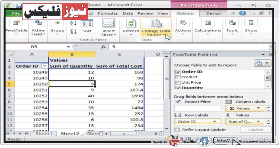
How to Modify the Pivot Table’s Data Source and Range
Excel’s pivot tables are an effective and flexible tool for analyzing and condensing huge datasets. They give consumers quick and straightforward access to data organization and filtering while offering insightful analytics. Using this tool, you can turn complicated data into insightful statistics. What happens though if you wish to modify the source and range in an Excel pivot table? For more information, keep reading.
Modifying the data source and range in a pivot table in Microsoft Excel is not difficult. Since spreadsheets are frequently updated with new information, you must update your pivot table in order to obtain accurate, up-to-date statistics.
Two typical scenarios for an updated dataset are as follows: Your dataset will either have new rows (or columns) of data added to it, or it will be modified in a brand-new spreadsheet. You should alter the data range in the first case and the data source in the second in order to update your pivot table.
In a pivot table, modify the date range, Let’s think about this You have numerous new entries added to your already existing dataset, and now need to change the data range in the pivot table. How to do it is as follows:
1. Launch the revised Excel workbook.
2. Pick any available cell in the pivot table.
3. From the top menu, select the PivotTable Analyse tab.
4. Choose the option to Change Data Source.
5. Choose the table or range you wish to analyze by typing in the box next to Table/Range or by clicking and dragging the mouse over the desired cell range.
The table/Range would be formatted as follows:
…[Sheet Name]$[Beginning Column]Beginning Row to Ending Column$[End Row]
For instance, the data in Sheet1’s cells A2 to P34 would be chosen by the text that follows:
Sheet1!$A$2:$P$34
6. Choose OK. The range of your pivot table has been modified.
Pivot Table Data Source Change
Suppose your new dataset is in a new worksheet. What then? Again, this is simple. Simply alter the pivot table’s data source. Take these actions:
1. Open the most recent version of your Excel spreadsheet.
2. Select an area of the pivot table by clicking.
3. From the top bar, select the PivotTable Analyse tab.
4. From this menu, select the Change Data Source option.
5. After the Move PivotTable window has opened, click the sheet name at the bottom of the Excel window to navigate to the sheet containing the new data set.
6. Choose the dataset you want to analyze by using the mouse to pick the desired range of the dataset’s cells or by typing the desired range into the Table/Range box.
Here is how to enter data:
…[Sheet Name]$[Beginning Column]Beginning Row to Ending Column$[End Row]
For instance, entering the following into the Table/Range box would pick the information in cells A1 to P29 on Sheet3:
7. Select OK. Your pivot table has just been revised.


